Operator learning · Approximation theory

Operator learning with optimal sampling

Learning an operator from finitely many input-output pairs requires choosing both an approximation space and a way to sample the inputs. We study these choices together through weighted least squares in a Bochner $L^2$ space, where the input measure determines how approximation error is measured. An operator-level Christoffel function connects the approximation space to sampling measures and weights that make recovery stable.

We construct linear and polynomial operator spaces, establish density under assumptions on the input measure, and describe how to sample from the associated Christoffel measures. Our finite-sample bounds separate best-approximation error from the error introduced by fitting from data. For suitable product spaces with full-field observations, the empirical Gram matrix reduces to repeated scalar blocks, so the number of samples sufficient for stability is independent of the output dimension.
With Matthew Lowery, John D. Jakeman, Zachary Morrow, Akil Narayan, and Varun Shankar.

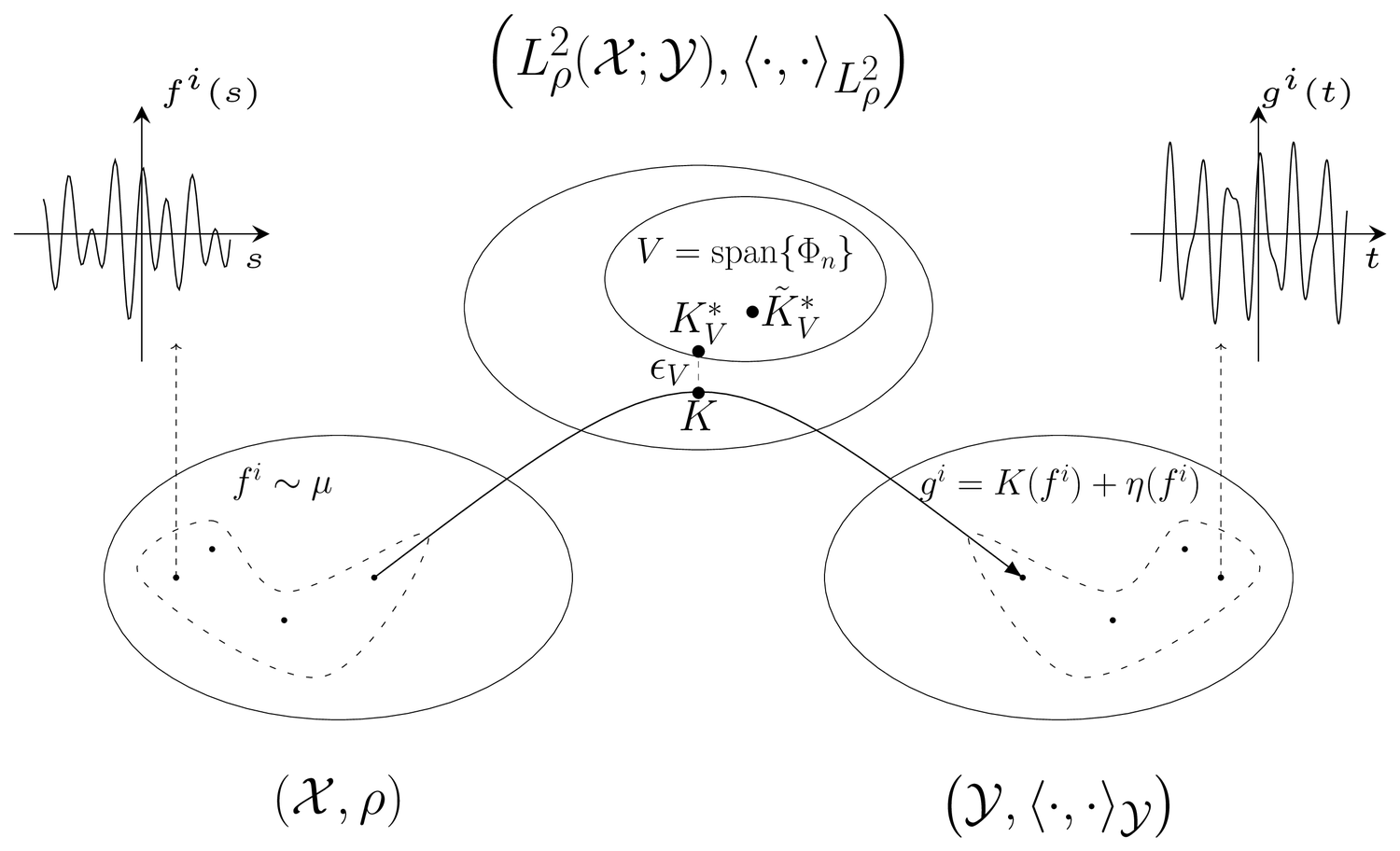
Schematic of the least-squares problem relating sampled inputs, noisy outputs, and the approximation space of operators.
Inputs are sampled from a measure adapted to the operator space $V$. The diagram distinguishes the best-approximation error in $V$ from the error introduced by fitting from finite data.

Uncertainty quantification · Gaussian measures

Uncertainty quantification for operator learning

A finite-dimensional operator approximation leaves a residual that the fitted coefficients do not describe. We study how additional observations can inform this residual through a Gaussian prior on the orthogonal complement of the approximation space. Defining the observation model requires care: point evaluation is not generally defined in a Bochner $L^2$ space. We establish conditions under which the prior assigns full measure to a Banach space where evaluation is continuous, and use Cameron–Martin theory to define the likelihood for noisy full-field observations.

The residual data are formed by subtracting the computed least-squares fit, so they also contain first-stage estimation error. We analyze how this error propagates through Gaussian conditioning and obtain finite-sample bounds on the posterior expected squared error of the complete approximation. Under compatible regularity assumptions, these bounds identify when the accuracy rate available from ideal residual observations is preserved.

With John D. Jakeman and Akil Narayan.

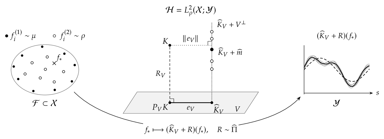
Schematic of the two-stage approximation, from sampled inputs through the approximation space to predicted outputs.
The two stages use independent input samples, shown as filled and open points. The residual correction lies in $V^\perp$, so the first-stage error within $V$ remains. At right: the first-stage prediction (dashed), posterior mean (solid), and posterior draws (grey) at a fixed input.

Quadrature · Probability

Constructive positive quadrature

Integrating a weighted least-squares approximation gives a quadrature rule exact on the approximation space. Even when the fit is well conditioned, however, the resulting weights need not be positive or yield a stable rule. We study these questions through the alignment between evaluation representers and the target functional, using probabilistic estimates to control how the scaled weights concentrate near their limiting values.

The analysis accommodates unbounded Christoffel functions and limiting weights that approach zero. Under suitable sampling and positivity assumptions, we obtain positive exact rules that can be reduced to at most $N$ nodes for an $N$-dimensional real approximation space, giving a constructive generalized Tchakaloff result. Additional tail assumptions provide weighted stability bounds for the rule before this reduction.

With Filip Bělík and Akil Narayan.

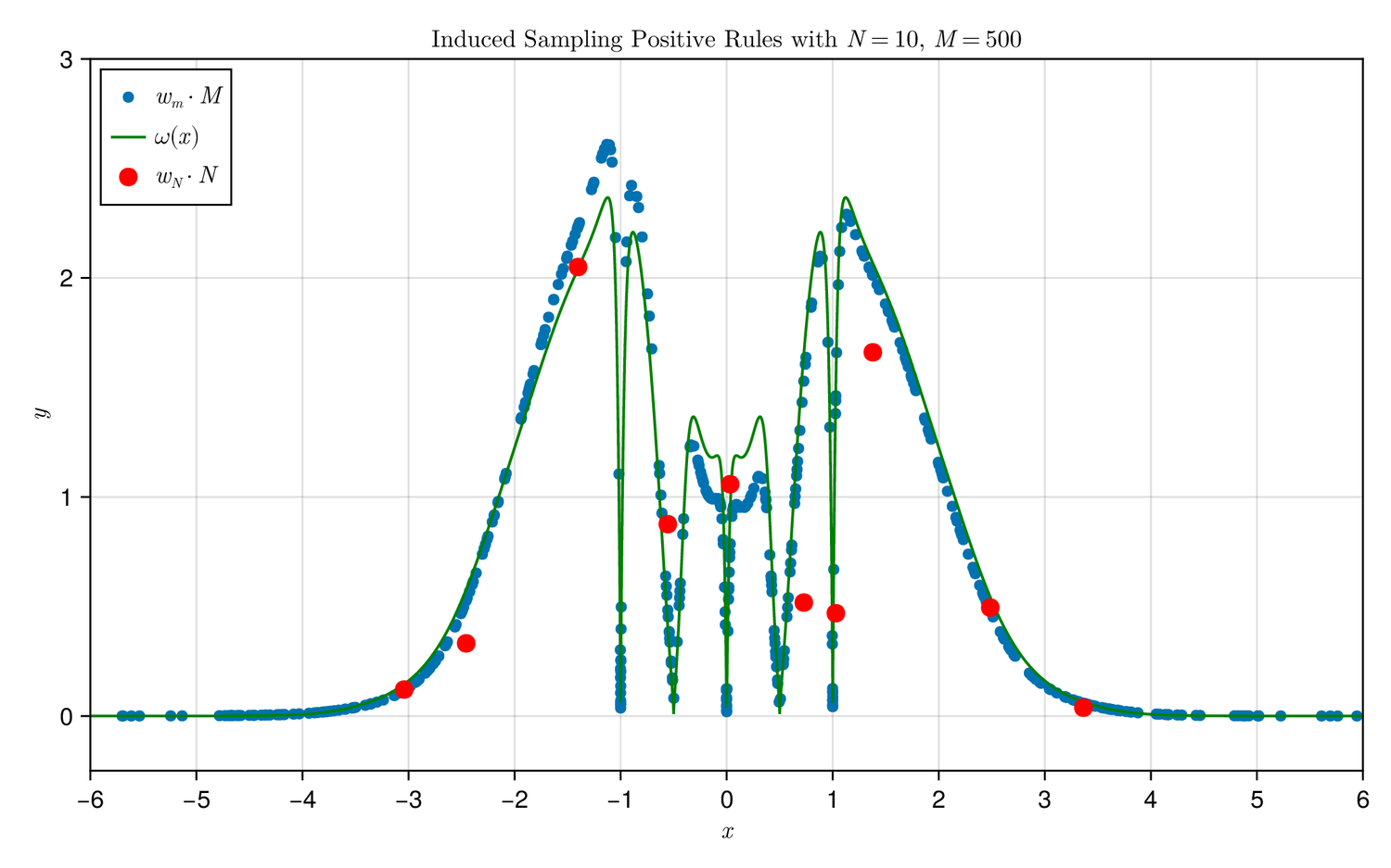
Quadrature weights from induced sampling clustering around their limiting curve, with the pruned positive rule marked in red.
A positive rule with 500 nodes is reduced to ten nodes while preserving exactness on the approximation space. For comparison, the original weights (blue) are multiplied by 500 and the reduced weights (red) by ten. Green shows the limiting scaled weights of the original rule.